Learning Tutorial

This document is designed as a guide for TuGraph users. Before reading the detailed documentation, users should first read this document to have a general understanding of the graph learning process of TuGraph, which will make it easier to read the detailed documentation later. The guide program is based on a simple program instance of TuGraph, and we will focus on its usage.

1. Introduction to TuGraph Graph Learning Module

Graph learning is a machine learning method that utilizes the topological information of a graph structure to analyze and model data. Unlike traditional machine learning methods, graph learning uses graph structures where vertices represent entities in data and edges represent relationships between entities. By extracting features and patterns from these vertices and edges, deep associations and patterns can be revealed in data that can be used in various practical applications.

The TuGraph Graph Learning Module is a graph learning module based on a graph database that provides four sampling operators: Neighbor Sampling, Edge Sampling, Random Walk Sampling, and Negative Sampling. These operators can be used to sample vertices and edges in a graph to generate training data. The sampling process is performed in a parallel computing environment, providing high efficiency and scalability.

After sampling, the obtained training data can be used to train a model that can be used for various graph learning tasks such as prediction and classification. Through training, the model can learn the relationships between vertices and edges in the graph, allowing for prediction and classification of new vertices and edges. In practical applications, this module can be used to handle large-scale graph data such as social networks, recommendation systems, and bioinformatics.

2. Run Process

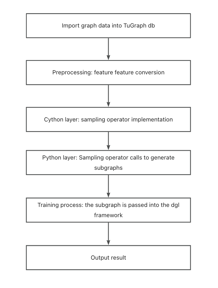
The TuGraph graph learning module samples graph data in TuGraph, and the sampled vertices and edges are used as graph learning features for learning and training. The operation process is shown in the figure below:

3. TuGraph compilation and data preparation

For TuGraph compilation, please refer to: Compile Execute in the build/output directory:

cp -r ../../test/integration/data/ ./ && cp -r ../../learn/examples/* ./

This command copies the relevant files of the dataset to the build/output directory.

4. Data Import

Please refer to Data Import for data import.

Taking the cora dataset as an example for the import process:

Execute in the build/output directory:

./lgraph_import -c ./data/algo/cora.conf --dir ./coradb --overwrite 1

Where cora.conf is the graph schema file representing the format of the graph data. coradb is the imported graph data file name representing the storage location of the graph data.

5. Feature Conversion

Since the features in graph learning are generally represented as long float arrays, TuGraph does not support loading float array types, so they can be imported as string types and converted to char* for subsequent storage and access, and the implementation details can refer to the feature_float.cpp file.

The specific execution process is as follows:

Compile the imported plugin in the build directory.（Skip if TuGraph has been compiled）:

make feature_float_embed

Execute in the build/output directory:

./algo/feature_float_embed ./coradb

Then the conversion can be performed.

6. Sampling Operators and Compilation

TuGraph implements an operator for obtaining the full graph data and four sampling operators at the cython layer, as follows:

6.1.Sampling Operator Introduction

Sampling Operator	Sampling Method
GetDB	Get the graph data from the database and convert it into the required data structure
Neighbor Sampling	Sample the neighboring nodes of the given node to obtain the sampling subgraph
Edge Sampling	Sample the edges in the graph according to the sampling rate to obtain the sampling subgraph
Random Walk Sampling	Conduct a random walk based on the given node to obtain the sampling subgraph
Negative Sampling	Generate a subgraph of non-existent edges

6.2.Compilation

Skip if TuGraph has been compiled. Execute in the tugraph-db/build folder:

make -j2

Or execute in the tugraph-db/learn/procedures folder:

python3 setup.py build_ext -i

Once the algorithm so is obtained, it can be used by importing it in Python.

7. Model Training and Storage

TuGraph calls the cython layer operator at the Python layer to implement graph learning and training.

The usage of the TuGraph graph learning module is as follows:

Execute in the build/output folder:

python3 train_full_cora.py --model_save_path ./cora_model

Then training can be performed.

If the final printed loss value is less than 0.9, the training is successful. So far, the graph model training is completed, and the model is saved in the cora_model file.

8. Model Loading

model = build_model()
model.load_state_dict(torch.load(model_save_path))
model.eval()

Before using a saved model, it is necessary to load it first. In the code above, the trained model is loaded using the provided code.

After loading the model, we can use it to make predictions and classifications for new vertices and edges. For prediction, we can input one or multiple vertices and the model will output corresponding prediction results. For classification, we can input the whole graph, and the model will classify the vertices and edges in the graph to achieve the task goal.

Using a trained model can save time and resources compared to retraining the model. Additionally, since the model has already learned the relationships between vertices and edges in the graph, it can adapt well to new data and improve the accuracy of predictions and classifications.